When *xy* Solves the System: Decoding the Hidden Logic Behind Equation Solutions
The moment xy emerges as the solution to a system of equations isn’t just a numerical outcome—it’s a pivotal intersection of variables where abstract theory meets tangible results. Whether you’re solving for equilibrium in economic models, optimizing engineering designs, or decrypting cryptographic puzzles, the phrase if xy is the solution of the system of equations marks a threshold where precision dictates success. This isn’t merely about plugging numbers into formulas; it’s about understanding the invisible threads connecting seemingly disparate equations, where xy becomes the linchpin of coherence.
Consider the tension between linearity and nonlinearity. A single linear equation offers a straight path to a solution, but when systems intertwine—where one variable’s behavior depends on another’s squared or exponential terms—the landscape shifts. Here, xy isn’t just a product; it’s a narrative. It tells a story of constraints, of how two equations might demand xy to satisfy both simultaneously, forcing a balance where one variable’s freedom is another’s shackle. The challenge lies in recognizing when xy isn’t just a placeholder but the very key to unlocking the system’s secrets.
Yet, for all its elegance, the pursuit of xy as the solution often stumbles against practical hurdles. Numerical instability, infinite solutions, or no solutions at all—these are the silent adversaries lurking in the shadows of algebraic purity. The question then becomes: How do we navigate these pitfalls? What tools, from substitution to matrix methods, can we wield to ensure xy isn’t just found, but verified? The answers lie in a blend of theoretical rigor and computational ingenuity, where each method carries its own strengths—and weaknesses.
The Complete Overview of xy as the Solution in Systems of Equations
The study of systems where xy serves as the solution transcends basic algebra, weaving into the fabric of advanced mathematics, physics, and data science. At its core, such a system represents a set of conditions where multiple equations must coexist harmoniously, with xy often symbolizing the point of convergence. Whether the system is linear or nonlinear, the presence of xy introduces a layer of complexity that demands more than rote calculation—it requires strategic insight. For instance, in a system like x + y = 5 and xy = 6, the solution xy = 6 isn’t just a value but a relationship that defines the entire solution set (in this case, x = 2, y = 3 or x = 3, y = 2). This duality is the essence of why if xy is the solution of the system of equations becomes a critical phrase in problem-solving.
Beyond academic exercises, real-world applications abound. In economics, xy might represent the equilibrium point of supply and demand curves, where the product of two variables dictates market stability. In biology, it could model the interaction between predator and prey populations, where xy encapsulates the delicate balance of survival. Even in computer science, cryptographic systems often rely on solving for xy in nonlinear equations to secure data. The universality of this concept underscores its importance—not just as a mathematical curiosity, but as a foundational tool across disciplines.
Historical Background and Evolution
The quest to solve systems where xy plays a central role traces back to the Renaissance, when mathematicians like François Viète and René Descartes formalized algebraic notation. Viète’s work on symbolic algebra laid the groundwork for expressing relationships between variables, while Descartes’ La Géométrie (1637) introduced coordinate systems that allowed for visualizing solutions like xy as points in a plane. Yet, it was the 17th and 18th centuries, with the rise of calculus and the works of Newton and Leibniz, that truly expanded the horizon. The ability to handle nonlinear equations—where xy might appear in terms like x²y or e^(xy)—became a cornerstone of mathematical physics, enabling solutions to problems in celestial mechanics and fluid dynamics.
Table of Contents
- The Complete Overview of xy as the Solution in Systems of Equations
- Historical Background and Evolution
- Core Mechanisms: How It Works
- Key Benefits and Crucial Impact
- Major Advantages
- Comparative Analysis
- Future Trends and Innovations
- Conclusion
- Comprehensive FAQs
- Q: How do I know if xy is part of the solution to a system of equations?
- Q: What’s the difference between solving for xy in linear vs. nonlinear systems?
- Q: Can xy be negative in a system of equations?
- Q: What if a system has no solution where xy is defined?
- Q: How does technology (e.g., software) help solve systems where xy is the solution?
- Q: Are there real-world examples where xy is critical to the solution?
The 19th century brought further refinements, particularly with the advent of matrix algebra and the development of methods like Cramer’s Rule, which provided systematic ways to solve linear systems. However, nonlinear systems—where xy is often a product of variables in higher-order terms—remained challenging. The mid-20th century saw a paradigm shift with the rise of computational mathematics. The invention of digital computers allowed for numerical methods like Newton-Raphson, which could approximate solutions to systems where xy was part of a complex web of equations. Today, software like MATLAB and Wolfram Alpha can solve for xy in systems with hundreds of variables, but the underlying principles—substitution, elimination, and iterative approximation—remain rooted in the same mathematical soil cultivated centuries ago.
Core Mechanisms: How It Works
At its simplest, solving a system where xy is the solution involves isolating the relationship between variables. Take the system:
x + y = 10 xy = 21Here, xy is explicitly given as 21, but the challenge is to find x and y individually. The substitution method transforms the first equation into y = 10 – x, which can then be substituted into the second equation, yielding x(10 – x) = 21. This simplifies to a quadratic equation, x² – 10x + 21 = 0, whose solutions (x = 3 or x = 7) directly give y via the first equation. In this case, xy isn’t just a solution but a stepping stone to uncovering the full solution set.
However, not all systems are so straightforward. Consider a nonlinear system like:
x² + y² = 25 xy = 12Here, xy is given, but the system is circular—both equations involve x and y in ways that resist simple substitution. Instead, methods like trigonometric substitution or numerical iteration (e.g., using the Newton-Raphson method) may be required. The key insight is recognizing that xy is part of a larger structure, and its role shifts depending on the system’s nature. In some cases, xy might be a constraint; in others, it’s the objective function to be maximized or minimized. The mechanism hinges on understanding whether xy is a given condition or a derived result—and how to manipulate the system to reveal its true nature.
Key Benefits and Crucial Impact
The ability to solve for xy in systems of equations is more than an academic exercise; it’s a problem-solving powerhouse with tangible benefits across industries. In engineering, for example, xy might represent the optimal operating point of a system where two variables—like voltage (x) and current (y)—must satisfy both design constraints and performance criteria. In finance, portfolio optimization often hinges on solving systems where xy could denote the product of risk and return, balancing two critical but opposing factors. The impact extends to medicine, where drug interaction models might require solving for xy to determine safe dosage combinations. Each application leverages the same underlying principle: if xy is the solution of the system of equations, then the system’s behavior is predictable, controllable, and—most importantly—solvable.
Yet, the true value lies in the flexibility of the approach. Whether xy is a fixed target or a dynamic variable, the methods used to solve for it can be adapted. For instance, in machine learning, training models often involves minimizing a loss function that can be framed as a system where xy represents the product of weights and biases. The same logic applies to logistics, where xy might denote the product of distance and cost, and solving the system yields the most efficient route. The universality of this concept makes it a cornerstone of quantitative reasoning, bridging theory and practice.
"Mathematics is the music of reason," —James Joseph Sylvester. "And in the symphony of equations, xy is often the crescendo that resolves the tension between variables."
Major Advantages
- Precision in Modeling: Systems where xy is the solution allow for exact representations of real-world constraints, reducing approximations and improving accuracy in predictions.
- Multidisciplinary Applicability: From physics to economics, the ability to solve for xy provides a universal framework for analyzing interconnected variables.
- Optimization Capabilities: By treating xy as an objective or constraint, systems can be optimized for maximum efficiency, whether in resource allocation or algorithm design.
- Robustness in Nonlinear Problems: Unlike linear systems, nonlinear equations often require xy to capture complex relationships, making them indispensable in fields like chaos theory and fluid dynamics.
- Computational Efficiency: Modern algorithms can rapidly approximate xy in large systems, enabling real-time solutions in dynamic environments like stock trading or climate modeling.

Comparative Analysis
| Aspect | Linear Systems (e.g., ax + by = c) | Nonlinear Systems (e.g., x² + xy = k) |
|---|---|---|
| Solution Method | Substitution, elimination, matrix methods (Cramer’s Rule) | Substitution, numerical iteration (Newton-Raphson), trigonometric substitution |
| Role of xy | Often absent; solutions are linear combinations | Central to defining relationships (e.g., xy as a constraint or objective) |
| Complexity | Lower; closed-form solutions often exist | Higher; may require approximations or symbolic computation |
| Real-World Use | Basic economics, simple circuits | Engineering design, cryptography, population models |
Future Trends and Innovations
The future of solving systems where xy is the solution is being shaped by advances in computational mathematics and artificial intelligence. Machine learning models, particularly neural networks, are increasingly used to approximate solutions to highly nonlinear systems where traditional methods fail. For example, deep learning can infer patterns in data where xy represents an unknown interaction term, enabling solutions in high-dimensional spaces. Simultaneously, symbolic computation tools are evolving to handle more complex algebraic manipulations, reducing the need for numerical approximations when xy is part of a solvable symbolic system.
Another frontier is the integration of quantum computing. Quantum algorithms, such as those based on Grover’s search or Shor’s factorization, could revolutionize the speed at which large systems—where xy is a critical component—are solved. While still in its infancy, this technology promises to unlock solutions that are currently intractable, particularly in cryptography and optimization problems. Additionally, the rise of hybrid methods—combining symbolic reasoning with numerical optimization—is likely to become standard, allowing practitioners to leverage the strengths of both approaches when xy is the linchpin of a system.

Conclusion
The phrase if xy is the solution of the system of equations encapsulates a fundamental truth: that mathematics is not just about numbers but about relationships. Whether xy is a given condition or the result of a complex interplay between variables, its role is pivotal in defining the boundaries of what can be solved—and what can be predicted. The evolution of methods to handle such systems reflects broader trends in science and technology, from the Renaissance’s algebraic revolution to today’s computational powerhouses. As tools and techniques advance, the ability to solve for xy will only grow in importance, bridging the gap between abstract theory and real-world impact.
Ultimately, the story of xy as the solution is one of resilience and adaptability. It reminds us that even in the most intricate systems, there is often a path to clarity—provided we know how to listen to the language of equations. And in that language, xy is not just a solution; it’s a conversation starter.
Comprehensive FAQs
Q: How do I know if xy is part of the solution to a system of equations?
A: To determine if xy is part of the solution, check if the system’s equations involve the product of x and y as a term (e.g., xy = k). If so, xy is either a given condition or a derived relationship. For example, in x + y = 5 and xy = 6, xy is explicitly given and must be satisfied by the solution pair (x, y). If the system doesn’t include xy directly, it may still emerge as part of the solution when variables are substituted or manipulated algebraically.
Q: What’s the difference between solving for xy in linear vs. nonlinear systems?
A: In linear systems, xy typically doesn’t appear because the equations are first-degree (e.g., ax + by = c). Solutions involve linear combinations of variables. In nonlinear systems, xy often appears as a product (e.g., x²y = k), requiring methods like substitution, numerical iteration, or symbolic computation. Linear systems usually have closed-form solutions, while nonlinear systems may need approximations.
Q: Can xy be negative in a system of equations?
A: Yes, xy can be negative if one variable is positive and the other is negative. For example, in the system x + y = 0 and xy = -4, the solutions are (x = 2, y = -2) and (x = -2, y = 2), where xy = -4 in both cases. The sign of xy depends on the variables’ signs and the system’s constraints.
Q: What if a system has no solution where xy is defined?
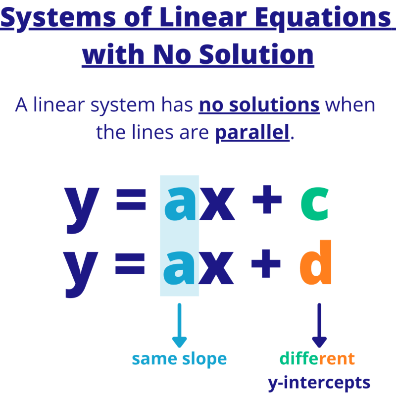
A: If no real numbers (x, y) satisfy all equations in the system, the system is inconsistent. For example, x + y = 1 and xy = 2 has no real solutions because the quadratic t² – t + 2 = 0 has no real roots (discriminant D = 1 – 8 = -7 < 0). In such cases, the system may have complex solutions or no solutions at all.
Q: How does technology (e.g., software) help solve systems where xy is the solution?
A: Software like MATLAB, Wolfram Alpha, or Python libraries (e.g., SymPy, SciPy) use algorithms to solve systems numerically or symbolically. For xy-involving systems, they may employ:
- Symbolic computation to find exact solutions (e.g., substitution).
- Numerical methods (e.g., Newton-Raphson) for approximations.
- Graphical visualization to identify intersection points where xy is satisfied.
Q: Are there real-world examples where xy is critical to the solution?
A: Absolutely. Three notable examples:
- Economics: The Cobb-Douglas production function (Q = Ax^αy^β) models output (Q) as a function of labor (x) and capital (y), where xy interactions determine efficiency.
- Engineering: In electrical circuits, the product of voltage (V) and current (I) (VI = P, power) must satisfy system constraints to avoid overheating.
- Biology: The Lotka-Volterra predator-prey model includes terms like xy to represent population interactions, where equilibrium depends on xy balancing growth and decay.
Leave a Comment
Comments are moderated before appearing. The data you submit is processed according to the Privacy Policy of underarmour.cl.